home

PDF (letter size)

CDF Mathematica file (download to run on your PC with Mathematica free player)

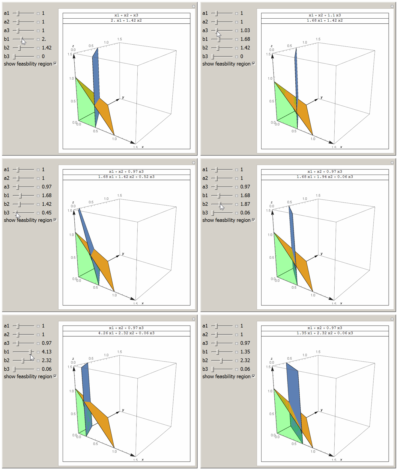
This small animation shows the feasibility region and the the intersection line between \(a_1 x_1 + a_2 x_2 + a_3 x_3= 1\) and \(b_1 x_1 + b_2 x_2 + b_3 x_3 =1\) and with \(x_i \geq 0\). The light Green region is the one in which \(a_1 x_1 + a_2 x_2 + a_3 x_3 \leq 1\) and \(b_1 x_1 + b_2 x_2 + b_3 x_3 \leq 1\). The optimal solution will be on a vertix on the line of interesection between the two planes shown. Done for class HW.

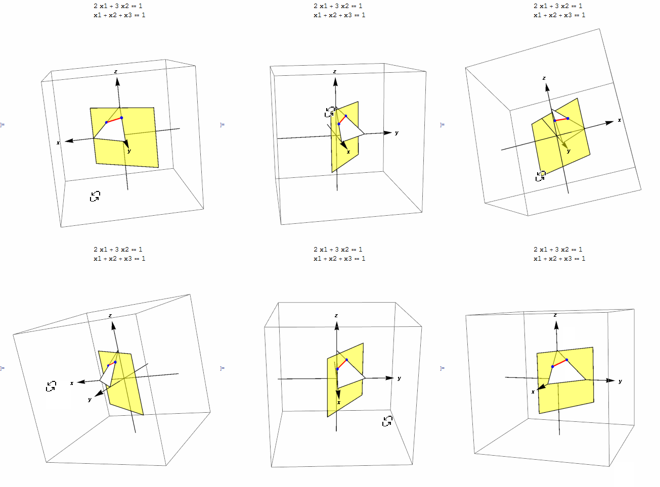
This small animation shows the feasibility region which is the intersection line between unit simplex given by \(x_1+x_2+x_3=1\) and plane \(2 x_1 + 3 x_2 = 1\).

Source code used to generate the first movie is

Manipulate[ 
 len = 1.5; 
 h = a1 x1 + a2 x2 + a3 x3; 
 g = b1 x1 + b2 x2 + b3 x3; 
 
 g1 = ContourPlot3D[{h == 1, g == 1}, {x1, 0, len}, {x2, 0, len}, {x3, 0, len}, 
   PlotRange -> {{0, len}, {0, len}, {0, len}}, 
   SphericalRegion -> True, MeshStyle -> {{Thick, Blue}}, Mesh -> {{0}}, 
   Lighting -> {{"Ambient", White}} 
   ]; 
 g2 = RegionPlot3D[h <= 1 && g <= 1, {x1, 0, len}, {x2, 0, len}, {x3, 0, len}, 
   PlotRange -> {{0, len}, {0, len}, {0, len}}, 
   SphericalRegion -> True, Mesh -> 0, 
   PlotStyle -> Directive[Green, Opacity[0.2]], 
   Lighting -> {{"Ambient", White}}]; 
 
 g3 = Graphics3D[{ 
    Arrow[{{0, 0, -len}, {0, 0, len}}], 
    Text[Style[z, Bold], {0, 0, 1.1 len}], 
    Arrow[{{0, -len, 0}, {0, len, 0}}], 
    Text[Style[y, Bold], {0, 1.1 len, 0}], 
    Arrow[{{-len, 0, 0}, {len, 0, 0}}], 
    Text[Style[x, Bold], {1.1 len, 0, 0}] 
    }]; 
 Grid[{ 
   {h}, 
   {g}, 
   { 
    If[showRegion, 
     Show[g1, g2, g3, ImageSize -> 400, ImagePadding -> 5] 
     , 
     Show[g1, g3, ImageSize -> 400, ImagePadding -> 5] 
     ] 
    }}, Frame -> All], 
 {{a1, 1, "a1"}, 0, 5, .01, Appearance -> "Labeled", ImageSize -> Tiny}, 
 {{a2, 1, "a2"}, 0, 5, .01, Appearance -> "Labeled", ImageSize -> Tiny}, 
 {{a3, 1, "a3"}, 0, 5, .01, Appearance -> "Labeled", ImageSize -> Tiny}, 
 {{b1, 2, "b1"}, 0, 5, .01, Appearance -> "Labeled", ImageSize -> Tiny}, 
 {{b2, 3, "b2"}, 0, 5, .01, Appearance -> "Labeled", ImageSize -> Tiny}, 
 {{b3, 0, "b3"}, 0, 5, .01, Appearance -> "Labeled", ImageSize -> Tiny}, 
 Row[{"show feasbility region ", Checkbox[Dynamic[showRegion]]}], 
 ControlPlacement -> Left 
 ]
 

Source code used to generate the second movie is

eq1 = 2 x1 + 3 x2 == 1; 
eq2 = x1 + x2 + x3 == 1; 
len = 2; 
g2 = Graphics3D[Simplex[{{1, 0, 0}, {0, 1, 0}, {0, 0, 1}}]]; 
g1 = ContourPlot3D[Evaluate@eq1, {x1, -1, 1}, {x2, -1, 1}, {x3, -1, 1}, 
   ContourStyle -> Directive[FaceForm[Yellow], Opacity[.5]], Mesh -> None, 
   Lighting -> {{"Ambient", White}}, Boxed -> True, Axes -> False]; 
g3 = Graphics3D[{ 
    Arrow[{{0, 0, -len}, {0, 0, len}}], Text[Style[z, Bold], {0, 0, 1.1 len}], 
    Arrow[{{0, -len, 0}, {0, len, 0}}], Text[Style[y, Bold], {0, 1.1 len, 0}], 
    Arrow[{{-len, 0, 0}, {len, 0, 0}}], Text[Style[x, Bold], {1.1 len, 0, 0}], 
    {Blue, Sphere[{0, 1/3, 2/3}, .05]}, 
    {Blue, Sphere[{1/2, 0, 1/2}, .05]}, 
    {Red, Thick, Line[{{0, 1/3, 2/3}, {1/2, 0, 1/2}}]} 
    }]; 
Grid[{{Column[{eq1, eq2}]}, 
  {Show[g1, g2, g3, PlotRange -> All, ImageSize -> 400, 
    SphericalRegion -> True]}}]
 

The following is the Mathematica notebook note.nb