2.2.1.3 Solved using first_order_ode_dAlembert

Entering first order ode dAlembert solver

\[\begin {aligned} x^{\prime }&=-\lambda x \end {aligned}\]

Let \(p=x^{\prime }\) the ode becomes

\begin{align*} p = -\lambda x \end{align*}

Solving for \(x\) from the above results in

\begin{align*} x &= -\frac {p}{\lambda }\tag {1A} \end{align*}

This has the form

\begin{align*} x&=t f(p)+g(p)\tag {*} \end{align*}

Where \(f,g\) are functions of \(p=x'(t)\). The above ode is dAlembert ode which is now solved.

Taking derivative of (*) w.r.t. \(t\) gives

\begin{align*} p &= f+(t f'+g') \frac {dp}{dt}\\ p-f &= (t f'+g') \frac {dp}{dt}\tag {2} \end{align*}

Comparing the form \(x=t f + g\) to (1A) shows that

\begin{align*} f &= 0\\ g &= -\frac {p}{\lambda } \end{align*}

Hence (2) becomes

\begin{align*} p = -\frac {p^{\prime }\left (t \right )}{\lambda }\tag {3} \end{align*}

The singular solution is found by setting \(\frac {dp}{dt}=0\) in the above which gives

\begin{align*} p = 0 \end{align*}

Solving the above for \(p\) results in

\begin{align*} p_{1} &=0 \end{align*}

Substituting these in (1A) and keeping singular solution that verifies the ode gives

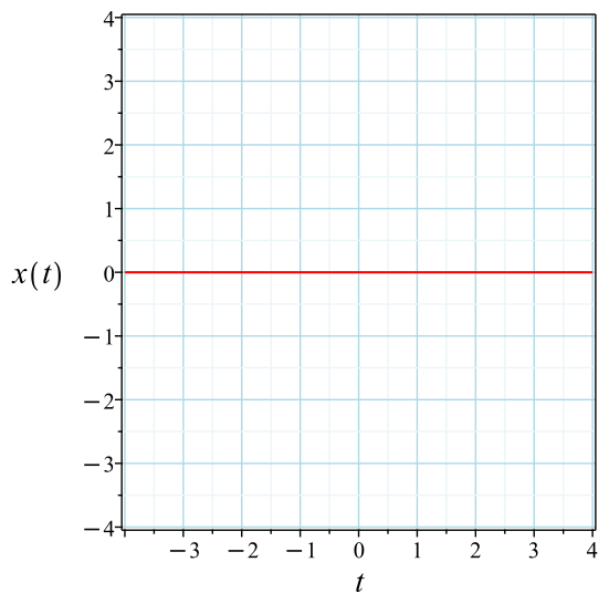
\begin{align*} x&=0 \end{align*}

The general solution is found when \( \frac { \mathop {\mathrm {d}p}}{\mathop {\mathrm {d}t}}\neq 0\) from eq. (3). This results in

\begin{align*} p^{\prime }\left (t \right ) = -p \left (t \right ) \lambda \tag {4} \end{align*}

This ODE is now solved for \(p \left (t \right )\). No inversion is needed.

Integrating gives

\begin{align*} \int -\frac {1}{p \lambda }d p &= dt\\ -\frac {\ln \left (p \right )}{\lambda }&= t +c_1 \end{align*}

Singular solutions are found by solving

\begin{align*} -p \lambda &= 0 \end{align*}

for \(p \left (t \right )\). This is because of dividing by the above earlier. This gives the following singular solution(s), which also has to satisfy the given ODE.

\begin{align*} p \left (t \right )&=0 \end{align*}

Solving for \(p\) from above gives

\[ p = -\frac {{\mathrm e}^{-c_1 \lambda -t \lambda }}{\lambda } \]

Substituing the above solution for \(p\) in \(x = -\frac {p}{\lambda }\) gives

\[ x = -\frac {{\mathrm e}^{-c_1 \lambda -t \lambda }}{\lambda } \]

Substituing the above solution for \(p\) in \(x = -\frac {p}{\lambda }\) gives

\[ x = 0 \]

Simplifying \(x = -\frac {{\mathrm e}^{-c_1 \lambda -t \lambda }}{\lambda }\) gives

\[ x = -\frac {{\mathrm e}^{-\lambda \left (t +c_1 \right )}}{\lambda } \]

Solutions plot

Summary of solutions found

\begin{align*} x&=0\\ x&=-\frac {{\mathrm e}^{-\lambda \left (t +c_1 \right )}}{\lambda } \end{align*}