home
PDF (letter size)
PDF (legal size)
Animation of swinging pendulum on spring
January 27, 2025 Compiled on January 27, 2025 at 4:32pm
Let original length of pendulum be \(L\) and extension at instance shown be \(x\) . The position vector of bob is
\[ \bar {r}=\left ( L+x\right ) \bar {b}_{1}\]
Hence the velocity vector is
\begin{align*} \left ( \frac {d}{dt}\bar {r}\right ) _{A} & =\left ( \frac {d}{dt}\bar {r}\right ) _{B}+\bar {\omega }\times \bar {r}\\ \bar {v}_{A} & =\left ( \frac {d}{dt}\left ( L+x\right ) \bar {b}_{1}\right ) _{B}+\bar {\omega }\times \left ( \left ( L+x\right ) \bar {b}_{1}\right ) \\ & =\dot {x}\bar {b}_{1}+\dot {\theta }\bar {b}_{3}\times \left ( \left ( L+x\right ) \bar {b}_{1}\right ) \\ & =\dot {x}\bar {b}_{1}+\dot {\theta }\left ( L+x\right ) \bar {b}_{2}\end{align*}
And the acceleration is
\[ \left ( \frac {d}{dt}\bar {v}\right ) _{A}=\left ( \frac {d}{dt}\bar {v}\right ) _{B}+\bar {\omega }\times \bar {v}\]
But
\begin{align} \left ( \frac {d}{dt}\bar {v}\right ) _{B} & =\frac {d}{dt}\left ( \dot {x}\bar {b}_{1}+\dot {\theta }\left ( L+x\right ) \bar {b}_{2}\right ) _{B}\nonumber \\ & =\ddot {x}\bar {b}_{1}+\left ( \ddot {\theta }\left ( L+x\right ) +\dot {\theta }\dot {x}\right ) \bar {b}_{2}\tag {2}\end{align}
And
\begin{align} \bar {\omega }\times \bar {v} & =\bar {\omega }\times \left ( \dot {x}\bar {b}_{1}+\dot {\theta }\left ( L+x\right ) \bar {b}_{2}\right ) \nonumber \\ & =\dot {\theta }\bar {b}_{3}\times \left ( \dot {x}\bar {b}_{1}+\dot {\theta }\left ( L+x\right ) \bar {b}_{2}\right ) \nonumber \\ & =\dot {\theta }\dot {x}\bar {b}_{2}+\dot {\theta }\dot {x}\bar {b}_{2}-\dot {\theta }^{2}\left ( L+x\right ) \bar {b}_{1}\tag {3}\end{align}
Substituting (2,3) into (1) gives the acceleration of the bob in frame \(A\) as
\begin{align*} \bar {a}_{A} & =\ddot {x}\bar {b}_{1}+\ddot {\theta }\left ( L+x\right ) \bar {b}_{2}+\dot {\theta }\dot {x}\bar {b}_{2}+\dot {\theta }\dot {x}\bar {b}_{2}-\dot {\theta }^{2}\left ( L+x\right ) \bar {b}_{1}\\ & =\ddot {x}\bar {b}_{1}+\ddot {\theta }\left ( L+x\right ) \bar {b}_{2}+2\dot {\theta }\dot {x}\bar {b}_{2}-\dot {\theta }^{2}\left ( L+x\right ) \bar {b}_{1}\end{align*}
To obtain \(\bar {F}=m\bar {a}\) we now just need to find \(\bar {F}\) . The force on bob is given by just the weight and the spring force acting
on it. The spring force is proportional to spring coefficient \(k\) times the extension. \(F_{s}=-kx\) . Hence the force vector is
\[ \bar {F}=mg\cos \theta \bar {b}_{1}-mg\sin \theta \bar {b}_{2}-kx\bar {b}_{1}\]
Therefore the equation of motion is
\begin{align*} \bar {F} & =m\bar {a}\\ mg\cos \theta \bar {b}_{1}-mg\sin \theta \bar {b}_{2}-kx\bar {b}_{1} & =m\left ( \ddot {x}\bar {b}_{1}+\ddot {\theta }\left ( L+x\right ) \bar {b}_{2}+2\dot {\theta }\dot {x}\bar {b}_{2}-\dot {\theta }^{2}\left ( L+x\right ) \bar {b}_{1}\right ) \\ g\cos \theta \bar {b}_{1}-g\sin \theta \bar {b}_{2}-\frac {k}{m}x\bar {b}_{1} & =\ddot {x}\bar {b}_{1}+\ddot {\theta }\left ( L+x\right ) \bar {b}_{2}+2\dot {\theta }\dot {x}\bar {b}_{2}-\dot {\theta }^{2}\left ( L+x\right ) \bar {b}_{1}\end{align*}
Or, by equating each vector component
\begin{align*} \ddot {x}-\dot {\theta }^{2}\left ( L+x\right ) +\frac {k}{m}x & =g\cos \theta \\ \ddot {\theta }\left ( L+x\right ) +2\dot {\theta }\dot {x} & =-g\sin \theta \end{align*}
Or
\begin{align*} \ddot {x} & =\dot {\theta }^{2}\left ( L+x\right ) -\frac {k}{m}x+g\cos \theta \\ \ddot {\theta } & =-\frac {2\dot {\theta }\dot {x}}{L+x}-\frac {g}{L+x}\sin \theta \end{align*}
Let initial conditions be \(L=1,x\left ( 0\right ) =0.1,\dot {x}\left ( 0\right ) =0,\theta \left ( 0\right ) =20^{0},\dot {\theta }\left ( 0\right ) =.1\) (rad/sec).
We can now solve for \(x,\theta \) as function of time and make the animations. We can assume values for \(m,k\) and
\(g=9.81\) .
The solution will give \(x\left ( t\right ) ,\theta \left ( t\right ) \) . To plot the path, we need to express \(x\left ( t\right ) \) in frame \(A\) coordinates of course which is the
fixed frame. But this is easy, since the pendulum frame \(B\) is fixed at the base on the frame A
origin.
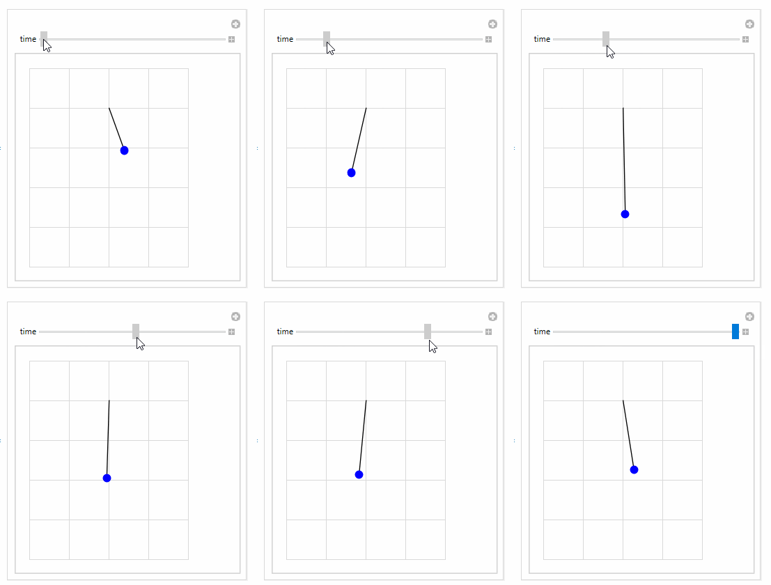
The following is plot of the solution using \(k=0.99,m=0.09\)
The following is a quick animation of the above
The following is the code used
(* Nasser M. Abbasi, Jan 25, 2025*)
SetDirectory [ NotebookDirectory []] L = 1;
k = .99;
m = .09;
g = 9.81;
ode1 = x '' [t] == z ' [t]^2*(L + x[t]) + g* Cos [z[t]] - k/m*x[t];
ode2 = z '' [t] == -2 z ' [t]*x ' [t]/(L + x[t]) - g* Sin [z[t]]/(L + x[t]);
IC = {x[0] == .1, x ' [0] == 0, z[0] == 20 Degree , z ' [0] == .1};
sol = NDSolve [{ode1, ode2, IC}, {x, z}, {t, 0, 100}]
Manipulate [ Module [{currentX, currentY},
currentX = (L + Evaluate [x[t0] /. sol])* Sin [ Evaluate [z[t0] /. sol]];
currentY = (L + Evaluate [x[t0] /. sol])* Cos [ Evaluate [z[t0] /. sol]];
Grid [{
{ Graphics [{
Line [{{0, 0}, {First@currentX, -First@currentY}}],
{ Blue , Disk [{First@currentX, -First@currentY}, .1]}
},
PlotRange -> {{-2, 2}, {-4, 1}}, GridLines -> Automatic ,
GridLinesStyle -> LightGray
]}}]
],
{{t0, 0, "time"}, 0, 10, .01},
TrackedSymbols :> {t0}
]

