Math 501 Project, Spring 2007. Project
review
Analysis of micro array gene expression
data for cancer detection
Last update June 3, 2007 by
Nasser Abbasi
To process microarray gene expression data samples, some of which is known to come from primary liver tumor tissues, and the rest from non-tumor liver samples, and then use PCA algorithm to generate significant features which represents the primary liver genes expressions.
This is followed by using these eigengenes (primary components) to detect the presence of tumor in any supplied gene expression samples and to analyze the effectiveness of these methods and suggest improvements and further investigations. As time permits, similar analysis will be carried on Bladder tumor gene expression.
Process over all work-flow
An overall work-flow diagram that shows the main components involved is illustrated in the following diagram. This diagram shows the input and output and data flow at a high level.
Data description
Some time was initially spent to understand clearly which data set to use for this analysis. For the Liver analysis, data used is that used by the Chen Xin, et all paper
This dataset includes 105 primary liver tumor samples, and 76 normal liver tumor samples.
I have a detailed description of the data here [HTML, WORD] which shows the GEO GSM accession ID for each sample, and the type of sample.
Originally, I started by using Matlab Bioinformatics toolbox (version 2.5). Using this toolbox, the liver primary tumor samples, and the non-tumor samples were downloaded from NCBI GEO database and saved locally for analysis. This is the log file of the download process.
Each sample was saved in a separate local file. Each one of these files contains the complete sample data with the meta data.
The following zip file contains all 181 sample files (105 primary tumors, 76 normal). [ZIP] (300MB). But these samples files contain all meta data and all the fields. (note: These files are not uploaded now due to large size). Use the smaller files below
I have compiled 2 other text files. The first text file called 'liverTumor.txt' contain the data from the primary tumor sample files, and the second text file called 'liverNormal.txt' which contains the data from the non-tumor sample files. These 2 files contain only the value reading from each of the 181 sample files.
There are 24,192 genes in each sample, and there are 105 tumor samples, and 76 normal samples.
Hence the file liverTumor.txt is a file that contains 24192 rows and 105 columns.
Similarly the file liverNormal.txt contains 24192 rows and 74 columns (76 samples - 2 samples found to have wrong number of genes)
These files can be easily read into matlab, and loaded into a variable of type matrix, using the load command as follows:
EDU>>
A=load('LiverTumor.txt');
size(A)
ans
=
24192 105
Here are the files to download [LiverTumor.txt , LiverNormal.txt ] (40 MB, 30 MB sizes).
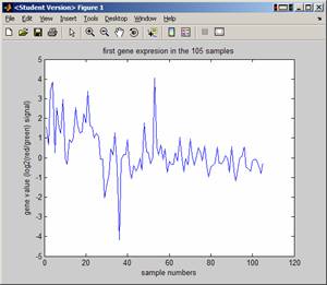
For example, to look at the 'first' gene, and to see what its value of expression across all 105 sample, do the following
EDU>> plot(A(1,:));
title('first gene expresion in the 105
samples');
EDU>> xlabel('sample
numbers'); ylabel('gene value (log2(red/green) signal)');

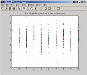
To look at first 10 genes across all samples, do
EDU>> plot(A(1:10,:),'.'); title('first 10 genes expresions in the 105 samples');
EDU>>

Microarray physical layout
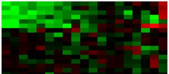
Using the platform record for each sample, it is possible to locate the physical spot location on the microarray for each gene. Given this coordinate system, and knowing the gene expression values, it is possible to recreate the red/green images of the microarray such as this one

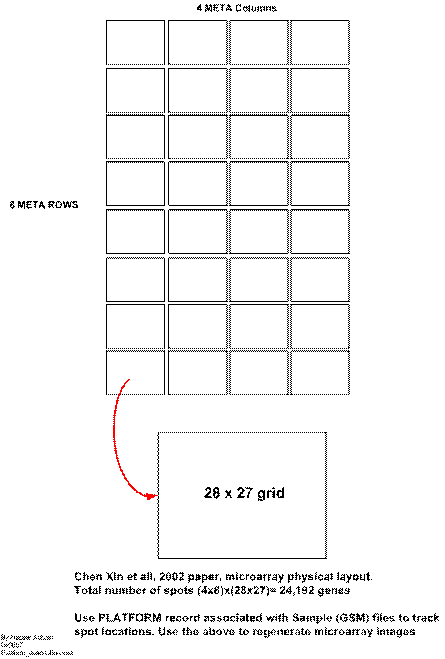
Microarray contains a grid that is build of blocks called meta blocks. Each meta block contains a grid within it where the spots are located. There are 32 meta blocks, arranged in 4 columns and 8 rows. The size of each meta block is 28x27, or 756 spots. Hence the total number of spots on one microarry is 24,192. This is illustrated in this diagram. And shown below
